Das Programm
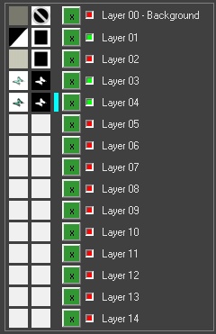
Das Programm besteht zentral aus einem Ebenen Modul. Auf diese Ebenen können Bilder und Masken geladen werden, die die Transparenz zur jeweils darunter liegenden Ebene bestimmen. Die Masken sind SW Bilder, in denen Weiß = deckend und Schwarz = transparent bedeutet. Grautöne sorgen je nach ihrem Wert für halbtransparente Überblendungen. Die Hintergrund-Ebene hat keine Maske. Der „X“ Button, schaltet einzelne Ebenen sichtbar oder unsichtbar. Das kleine rote oder grüne Feld zeigt in der Übersicht an, ob die entsprechende Ebene Pattern oder 2D Bild ist (rot = Pattern).

Den Bildern auf den einzelnen Ebenen können Eigenschaften zugewiesen werden. Eine Ebene kann Pattern, also Tiefenstruktur, sein oder als 2D Bitmap verwendet werden. Wenn eine Ebene „Pattern ist“, dann kann sie als pseudoskopisch (also nach vorne aus dem Bild heraustretend) definiert werden. Desweiteren können Pattern auf die Form der Linse maskiert (oder nicht) werden. Das Maß der Schrittweite bestimmt die Tiefe. Größere Schrittweiten sorgen für tiefere Bilder. Tiefere Bilder sind aber zugleich unschärfer, so dass Sie ein – von Fall zu Fall zu findendes – sinnvolles Maß nicht überschreiten sollten.

Abbildung der Eigenschaften einer 2D Bild Ebene.
Es gibt hier keine Optionen, weil das Bild vollflächig 2D auf seiner Ebene abgebildet wird. Die zum Bild geladene Maske bestimmt die Art und Weise und den Grad der Einblendung.

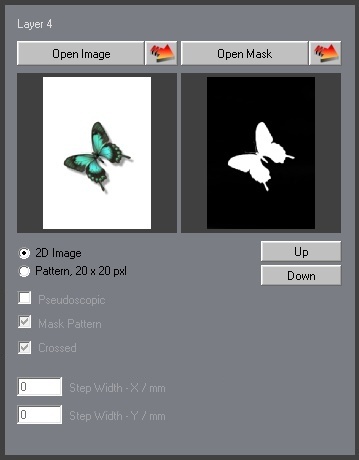
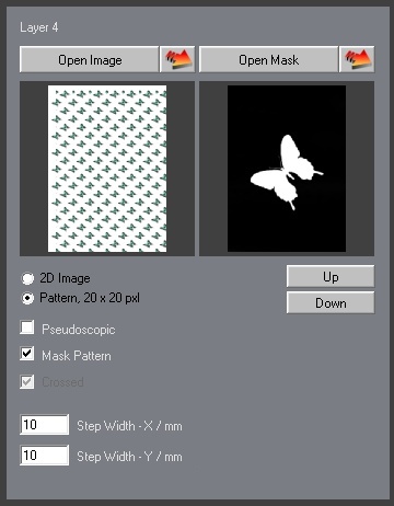
Abbildung der Eigenschaften einer Pattern Ebene.
Die Option „Mask Pattern“ ist aktiviert, damit das Bild auf Linsengröße begrenzt wird. Die „Pseudoscopic“ Option würde aktiviert, wenn dieses Pattern nicht in der Tiefe hinter, sondern im Raum vor der Bildebene dargestellt werden sollte. Unten ist die Schrittweite (und damit die Tiefe) eingestellt. Die roten Pfeiltasten führen zu einem Neuladen des auf dieser Ebene geladen Bildes bzw der Maske.

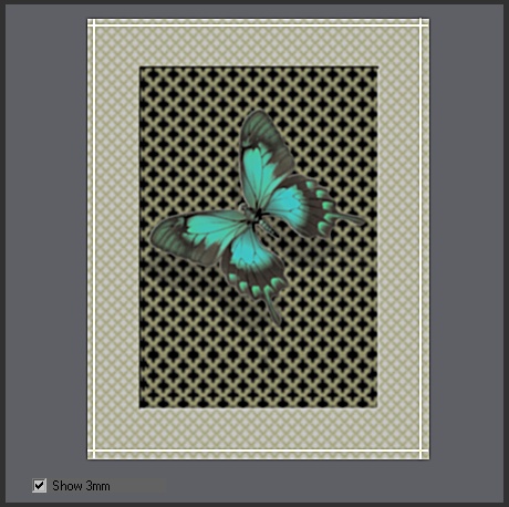
Das Ergebnis wird angezeigt.
Links unter dem Vorschaubild können Sie wählen, ob eine 3mm Beschnittmarkierung angezeigt werden soll oder nicht. Diese Marke wird nicht ins Ergebnis gerendert. Sie dient nur zu Ihrer Information.

Bevor Sie Ihr Design aufbauen, müssen Sie zuerst einige grundlegende Einstellungen machen. Geben Sie den LPI Wert für die X und die Y Richtung ein. Rechts der Eingabefelder ist eine Auswahlbox, die mit einigen gängigen Linsen vorkonfiguriert ist. Wählen Sie die LPI Einstellungen aus diese Box, wenn Ihr Material dort angeboten ist. Geben Sie weiterhin Druckbreite und Höhe in mm ein. Wählen Sie dann die Auflösung Ihres Ausgabegeräts. Darunter haben Sie die Wahl zwischen unterschiedlichen Linsentypen. Quantum kann Strukturen für alle Sorten von FlyEye-, Integral- und auch für Lenticularlinsen erstellen. Sobald Sie das erste Bild in eine der Ebenen geladen haben, sind diese Optionen nicht mehr verfügbar. Sie müssen diesen Setup also zuerst machen.

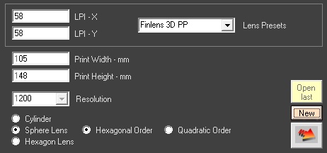
Wenn Sie Änderungen im Basis-Setup machen möchten, also z.B. die Größe ändern, dann klicken Sie auf die Schaltfläche „New“. Alle Bilder werden entfernt, die Setup Optionen sind wieder verfügbar und können geändert werden. Klicken Sie dann auf den Button mit dem roten Pfeil. Die Bilder Ihres Designs werden wieder geladen. Diese Vorgehensweise ist notwendig, weil die Werte des Setups und die programminterne Vorbereitung der Bilder sowie ihre Darstellung in der Vorschau miteinander verbunden sind.

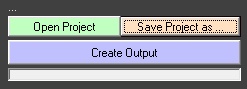
Rendern Sie den Output (TIF Format) durch Klick auf „Create Output“. Mit „Open und Save Project“ speichern Sie Ihr Design, um es zu einem späteren Zeitpunkt wieder aufrufen zu können.

Wenn Sie die „Auto Print Output“ aktivieren, dann wird nach jedem Rendering das Ergebnis an einen Drucker gesendet. Beim ersten Aufruf müssen Sie den Drucker und die Qualität wählen und einstellen. Nachfolgende Drucke gehen bei aktivierter Option automatisch an den Drucker. „Print last“ druckt das zuletzt gerenderte Bild.

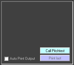
Der Button „Call Pitchtest“ ruft das Pitchtest Modul auf, mit dem Sie den Pitch-Wert von FlyEye- und Lenticular- Linsen mit angenäherter Genauigkeit bestimmen können.

So funktioniert es:.
Machen Sie von einem Linsenstück von ca 5×5 cm Größe einen Scan mit 1200 DPI Auflösung. Das können Sie mit jedem Flachbett Scanner tun. Legen Sie hinter die Linse ein Stück schwarzen Karton, um den Kontrast der Linsendarstellung im Scan zu erhöhen. Laden Sie den Scan dann in das Pitchtest Modul.

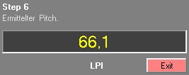
Das Pitchtest Modul leitet Sie in 6 Schritten an. Schritt 5 ist die eigentliche Messung. Das Programm fordert Sie auf, den roten Punkt genau ins Zentrum einer Linse (oder genau dazwischen) zu legen. Dann stellen Sie über einen Regler die schwarzen Punkte so ein, dass sie alle im Zentrum der nachfolgenden Linse sitzen (oder genau zwischen zwei benachbarten Linsen).

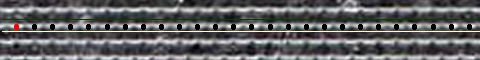
Das Ergebnis dieser Justage ist der Pitch der untersuchten Linse.

Wenn Sie Linsen ausmessen, die unter Umständen in X- und Y- Richtung unterschiedliche Pitch-Werte haben, dann müssen Sie den Scan für eine zweite Messung um 90 Grad drehen. Natürlich können Sie mit diesem Programm auch normale Lenticularlinsen ausmessen. Die Präzision der Messung liegt bei ca 0,2 LPI. Es ist also sinnvoll, den LPI Wert entweder mit einem gedruckten Pitchtest oder mit einer Reihe von Experimenten zu verfeinern. Bitte beachten Sie auch, dass der „optische Pitch“ und der hier gemessene „tatsächliche Pitch“ unterschiedlich sind. Das liegt an den optischen Eigenschaften der Linse in Bezug zur Betrachtungsdistanz und an verschiedenen Vorstufen- und drucktechnischen Umständen. Hier werden nur geometrische materielle Eigenschaften der Linse vermessen.